Excel Tip of the Week: Data Tables

Today’s topic is how to create a data table.

One of the things they teach us early in business school is to think broadly about our decisions. We are taught to think about best-case scenarios, worst-case scenarios, and everything in between. Excel can be very useful in exploring a number of different situations from a quantitative standpoint, and data tables are one of the main tools you can use to quickly and easily explore such scenarios.

Data tables allow you to see what the outcome would be if you changed one (or two) of your input variables. This means that instead of manually changing a cell one number at a time to see what would happen, you can list a large range of possible values for your input variable(s) and Excel will calculate the result for you.

Here is an example:

1. Download the example spreadsheet here
2. Make sure you are on the sheet titled “One Variable Data Table”
3. Using the 8% discount rate, we can see that if service was expanded the NPV for 5 years would be $1,147 209. However, we are not sure if 8% is correct. We would like to see what the NPV would be if the discount rate was as low as 6%, as high as 10%, and everything in between.
4. Notice in cells B9:B17 I have already created a range of values from 6% to 10% increasing at half percent intervals.
5. Now we can get down to business. Move your cursor to C8.
6. Press the “equals” button, then arrow up twice to cell C6 (the NPV formula) then hit “enter.”
7. Highlight cells B8:C17 – the box holding the data table.
8. PC: From the “Data” menu in the “Data Tools” section click “What-If Analysis” then “Data Table” (keyboard shortcut Alt → A → W → T)
9. Mac: From the “Data” menu in the “Analysis” section click “What-If” then “Data Table”
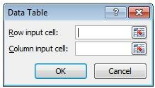
10. You should see the Data Table dialogue box pop up (see picture below)
11. Click into the “Column input cell” box and then click cell C5 (the discount rate)
12. Leave the “Row Input Cell” empty. Then click OK.

Notice that Excel has automatically placed a formula into each box that calculates the NPV given the different discount rates. A few things to keep in mind about data tables:

1. The number sitting at the top of the data table (in our example, cell C8) cannot be moved or deleted. But it looks weird sitting there, so I usually change its font color to match the background or hide the entire row.
2. You can’t delete a single row in a data table. If you need to alter the data table, you’ll have to remake it.
3. Sometimes calculations for Data Tables are turned off. Either change this using the calculation options (under the “Formulas” menu) or hit the F9 button to manually calculate. (CMD + = for a Mac)
4. Data tables can handle two variables and there is an advanced example showing you how to do that on the other tab in the example worksheet. Go try it out, you’ll be glad you did!