
A quick programming note before I jump in. There was no tip last week (totally undermining my title), and there was a flood of e-mails and complaints. Just kidding. I doubt anyone noticed. Nonetheless, I want to let you know the Excel tips might be less than weekly over the next few months since we are on summer break.
Today’s topic is absolute and relative cell references.
A key building block in formula writing is the ability to use absolute and relative cell references. I realize the term “absolute cell reference” makes you want to go to sleep. It sounds overly complex and difficult to grasp, but it is an EXTREMELY important concept for writing sound and efficient formulas.
 Heavy-Handed Metaphor!
If you don’t like the term “absolute cell reference” you can call it something different. Some people like to call it “locking” while others call it “anchoring.” Whatever you call it, make sure you know how to do it.
Here is a table explaining the four different ways a cell can be referenced:
| Reference Style | Meaning |
|---|---|
| A1 | Relative: This is the normal way to reference cells in Excel. Both the row and column will change if this formula is filled or copied elsewhere |
| $A$1 | Absolute: This cell will stay constant no matter where it is filled or copied |
| $A1 | Partial Reference (Column): This cell is only locked on the column, therefore the row number can change during a fill or copy, but the column cannot |
| A$1 | Partial Reference (Row): This cell is only locked on the row, therefore the column can change during a fill or copy, but the row cannot |
A quick note: When creating a formula you can hit the F4 key and cycle through all 4 cell reference options. (On a Mac the shortcut is CMD + T)
Now for a simple example (Click here to download the example spreadsheet) Below is a table showing the total forecasted sales for the months January through June (cell C1) and the forecasted seasonality of those sales (cells B4-B9). Using an absolute cell reference we will be able to build one formula which can help us fill in cells C4-C9.
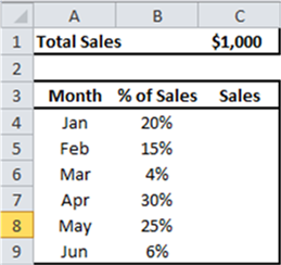
Here are the steps to creating the formula and completing the table:
1. Move the cursor into cell C4 and begin the formula by typing the equals sign: =
2. Arrow up to cell C1 then hit the F4 key (CMD+T on a Mac) to “lock” or “anchor” this cell
3. Hit the asterisk * for multiplication then arrow over to cell B4
4. Your formula should now read “=$C$1*B4” Hit the Enter button to complete the formula
5. The last step is to copy or fill the formula just created into cells C5-C9 (Bonus tip! Highlight cells C4-C9 then use the “fill down” shortcut: Ctrl + D to quickly copy and paste the formula into all the cells. It is the same on a Mac.)
Here is the finished product:
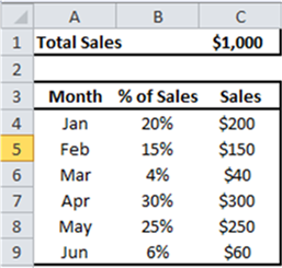
The big takeaway here is the ability to create one formula which performs 6 different calculations.
I would highly encourage you to open Excel and try this for yourself. This concept can be a bit confusing at first, but taking a “learn by doing” approach can go a long way toward understanding.
Questions or suggestions for future topics are gladly welcomed in the comments section.
THANK YOU!:)
Hello, your articles here Excel Tip of the Week: Absolute and Relative Cell References | OwenBloggers: Life as an MBA student at Vanderbilt University Owen Graduate School to write well, thanks for sharing!
Pingback: Excel Tip of the Week: RANK | OwenBloggers: Life as an MBA student at Vanderbilt University Owen Graduate School
Now the absolute cell references are Cmd + K
Pingback: Excel Tip of the Week: VLOOKUP & HLOOKUP | OwenBloggers: Life as an MBA student at Vanderbilt University Owen Graduate School
Pingback: Excel Tip of the Week: SUMIF | OwenBloggers: Life as an MBA student at Vanderbilt University Owen Graduate School